Attaching package: 'lubridate'
The following objects are masked from 'package:base':

    date, intersect, setdiff, union
── Attaching core tidyverse packages ──────────────────────── tidyverse 2.0.0 ──
✔ dplyr   1.1.4     ✔ stringr 1.5.1
✔ forcats 1.0.0     ✔ tibble  3.2.1
✔ purrr   1.0.2     ✔ tidyr   1.3.0
✔ readr   2.1.5
── Conflicts ────────────────────────────────────────── tidyverse_conflicts() ──
✖ dplyr::filter() masks stats::filter()
✖ dplyr::lag()    masks stats::lag()
ℹ Use the conflicted package (<http://conflicted.r-lib.org/>) to force all conflicts to become errors
Registered S3 method overwritten by 'quantmod':
  method            from
  as.zoo.data.frame zoo


Attaching package: 'forecast'


The following object is masked from 'package:astsa':

    gas


Registered S3 methods overwritten by 'ggfortify':
  method                 from
  autoplot.Arima         forecast
  autoplot.acf           forecast
  autoplot.ar            forecast
  autoplot.bats          forecast
  autoplot.decomposed.ts forecast
  autoplot.ets           forecast
  autoplot.forecast      forecast
  autoplot.stl           forecast
  autoplot.ts            forecast
  fitted.ar              forecast
  fortify.ts             forecast
  residuals.ar           forecast

Registered S3 methods overwritten by 'tsutils':
  method          from
  print.nemenyi   greybox
  summary.nemenyi greybox


Attaching package: 'reshape2'


The following object is masked from 'package:tidyr':

    smiths


Loading required package: zoo


Attaching package: 'zoo'


The following objects are masked from 'package:base':

    as.Date, as.Date.numeric


######################### Warning from 'xts' package ##########################
#                                                                             #
# The dplyr lag() function breaks how base R's lag() function is supposed to  #
# work, which breaks lag(my_xts). Calls to lag(my_xts) that you type or       #
# source() into this session won't work correctly.                            #
#                                                                             #
# Use stats::lag() to make sure you're not using dplyr::lag(), or you can add #
# conflictRules('dplyr', exclude = 'lag') to your .Rprofile to stop           #
# dplyr from breaking base R's lag() function.                                #
#                                                                             #
# Code in packages is not affected. It's protected by R's namespace mechanism #
# Set `options(xts.warn_dplyr_breaks_lag = FALSE)` to suppress this warning.  #
#                                                                             #
###############################################################################


Attaching package: 'xts'


The following objects are masked from 'package:dplyr':

    first, last
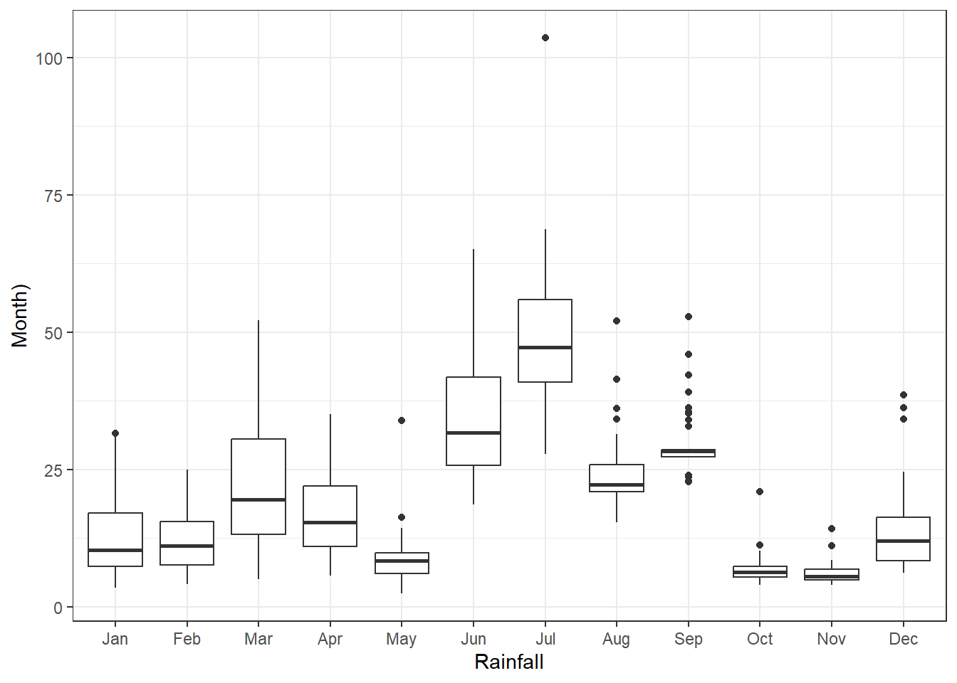
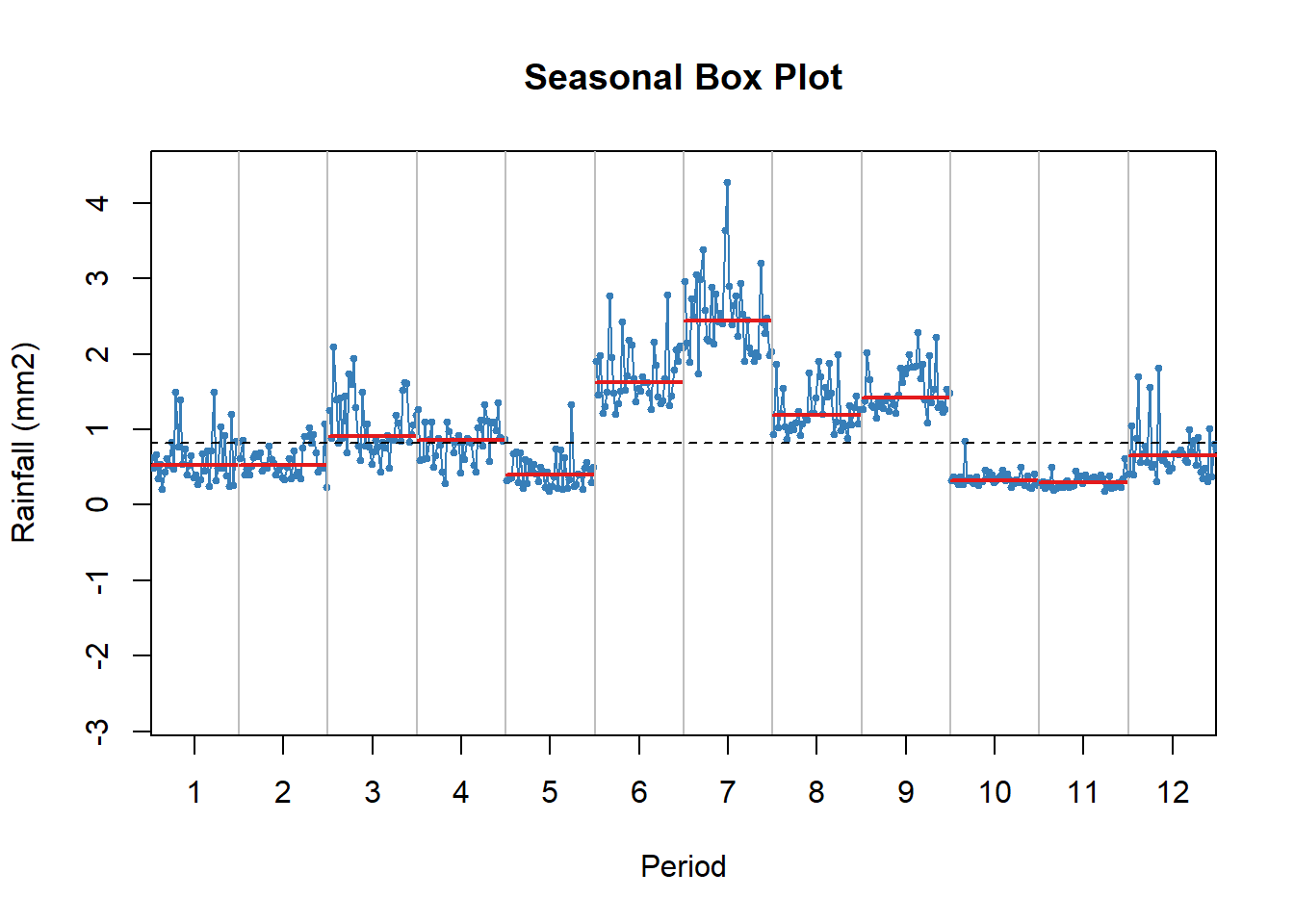
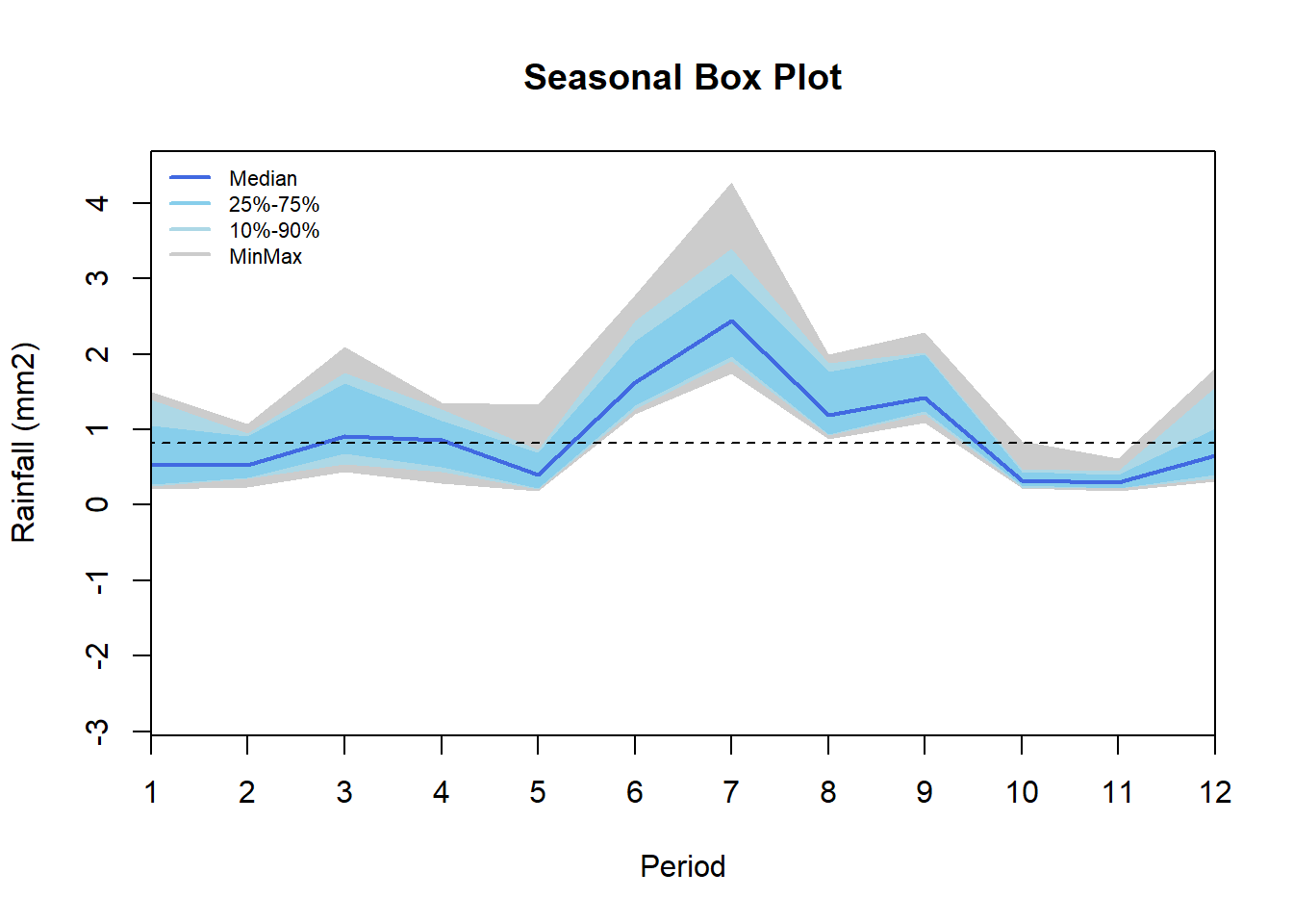
Sub-annual series
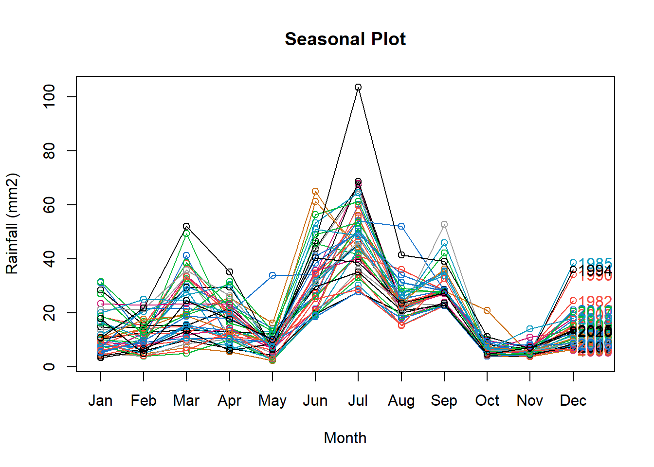
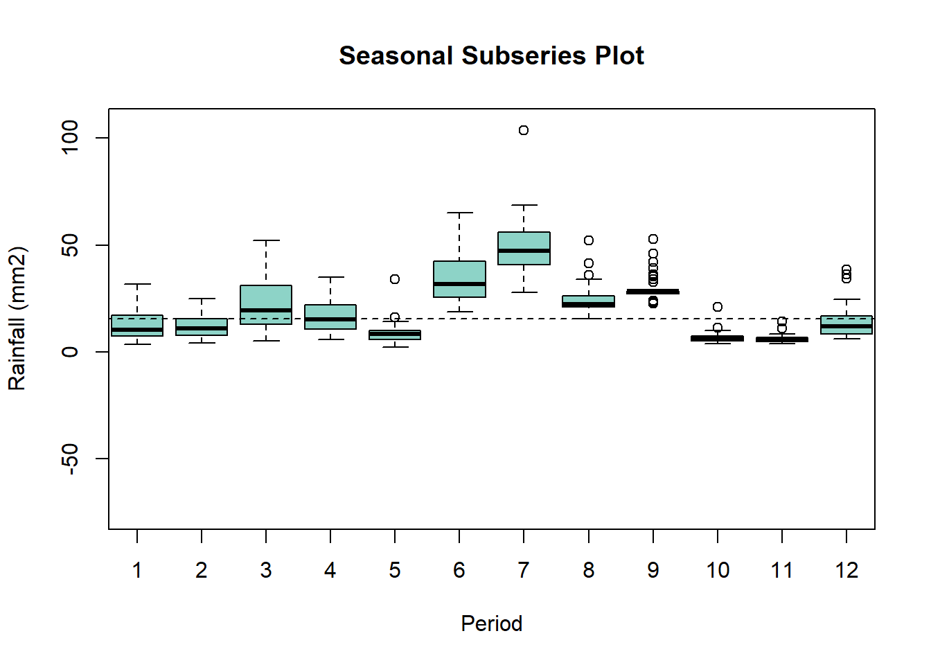
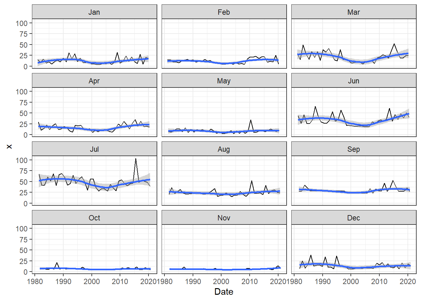
Rainfall data disaggregated per month showing highest rain in June and July and lowest in May October and November. Highest variability across years in found in March, June, July while lowest in September, October and November. Additionally distribution for the month of March(black line), June (green), and July (red) is shown.
Don't know how to automatically pick scale for object of type <ts>. Defaulting
to continuous.
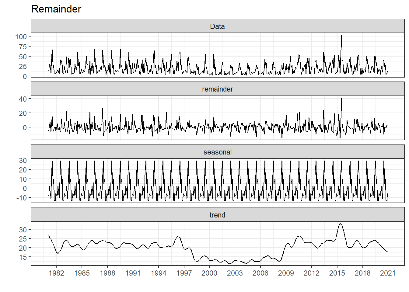
Decomposition
The strength of the trend and seasonal measured between 0 and 1, while “1” means there’s very strong of trend and seasonal occurred.
  Trend.Strength Seasonal.Strength
1            0.4               0.8
Seasonality analisys
Results of statistical testing
Presence of trend not tested.
Evidence of seasonality: TRUE  (pval: 0)
Results of statistical testing
Presence of trend not tested.
Evidence of seasonality: TRUE  (pval: 0)
Results of statistical testing
Presence of trend not tested.
Evidence of seasonality: TRUE  (pval: 0)
Warning in geom_smooth(method = loess, legend = FALSE): Ignoring unknown
parameters: `legend`
Don't know how to automatically pick scale for object of type <ts>. Defaulting
to continuous.
`geom_smooth()` using formula = 'y ~ x'
Forecasting
Train period from 1981 to 12.2015 and test period from 01.2016
Data it is checked against stationary state.
#######################
# KPSS Unit Root Test #
#######################

Test is of type: mu with 5 lags.

Value of test-statistic is: 0.3834

Critical value for a significance level of:
                10pct  5pct 2.5pct  1pct
critical values 0.347 0.463  0.574 0.739
###############################################
# Augmented Dickey-Fuller Test Unit Root Test #
###############################################

Test regression none


Call:
lm(formula = z.diff ~ z.lag.1 - 1 + z.diff.lag)

Residuals:
    Min      1Q  Median      3Q     Max
-31.409  -4.913   2.164  10.967  73.397

Coefficients:
           Estimate Std. Error t value Pr(>|t|)
z.lag.1    -0.19147    0.03094  -6.188 1.32e-09 ***
z.diff.lag -0.19143    0.04498  -4.256 2.51e-05 ***
---
Signif. codes:  0 '***' 0.001 '**' 0.01 '*' 0.05 '.' 0.1 ' ' 1

Residual standard error: 15.7 on 476 degrees of freedom
Multiple R-squared:  0.1507,    Adjusted R-squared:  0.1471
F-statistic: 42.23 on 2 and 476 DF,  p-value: < 2.2e-16


Value of test-statistic is: -6.1878

Critical values for test statistics:
      1pct  5pct 10pct
tau1 -2.58 -1.95 -1.62
Using 95% as confidence level, the null hypothesis (ho) for both of test defined as:
KPSS Test: Data are stationary at 10% confidence (value of 0.3834). DF Test:
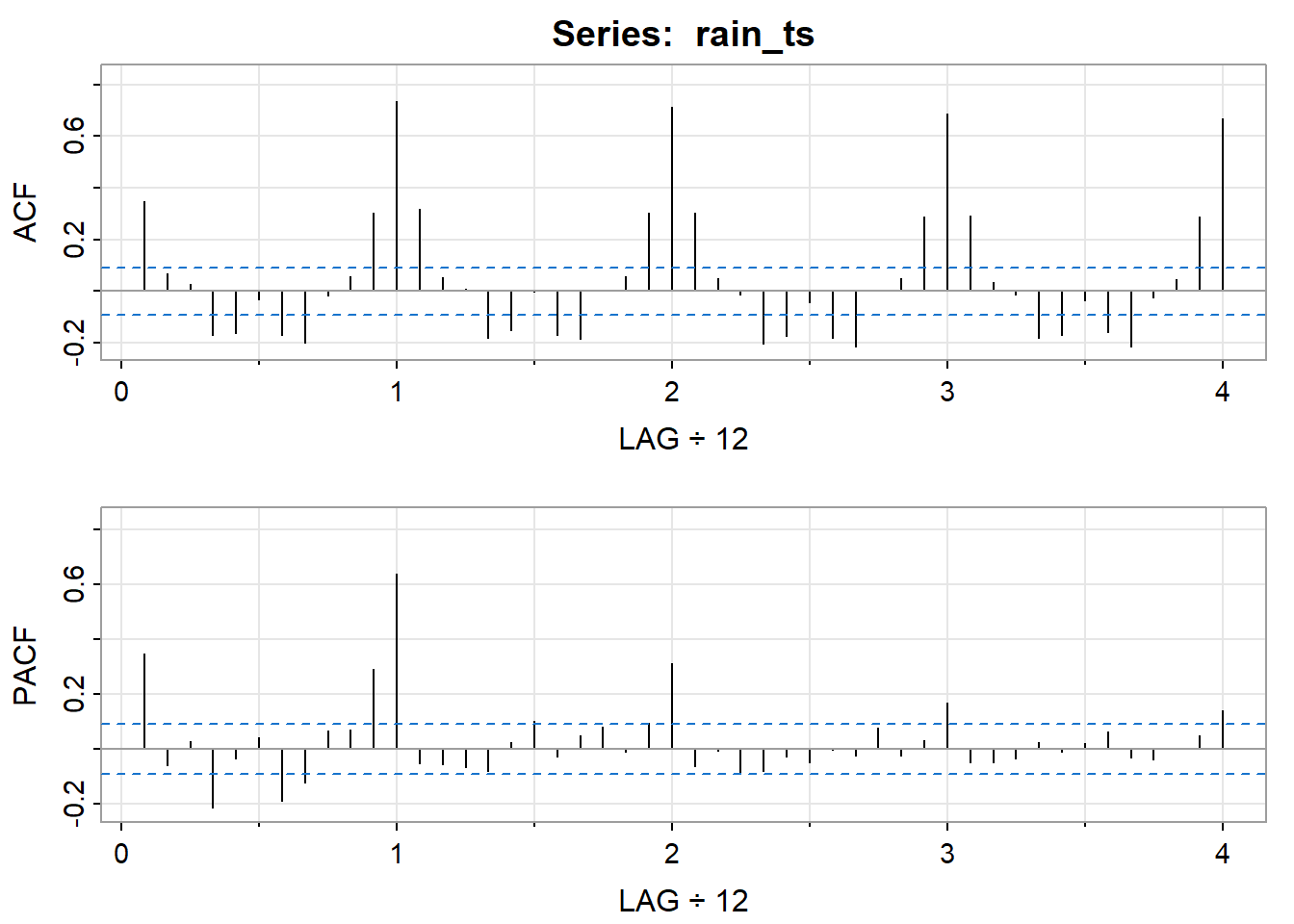
ARIMA analysis
Using different models for ARIMA.
     [,1]  [,2] [,3]  [,4]  [,5]  [,6]  [,7]  [,8]  [,9] [,10] [,11] [,12]
ACF  0.35  0.07 0.03 -0.17 -0.16 -0.03 -0.17 -0.20 -0.02  0.06  0.30  0.74
PACF 0.35 -0.06 0.03 -0.21 -0.04  0.04 -0.19 -0.12  0.06  0.07  0.29  0.64
     [,13] [,14] [,15] [,16] [,17] [,18] [,19] [,20] [,21] [,22] [,23] [,24]
ACF   0.32  0.05  0.01 -0.18 -0.15   0.0 -0.17 -0.19  0.01  0.06   0.3  0.71
PACF -0.05 -0.06 -0.07 -0.08  0.02   0.1 -0.03  0.05  0.08 -0.01   0.1  0.31
     [,25] [,26] [,27] [,28] [,29] [,30] [,31] [,32] [,33] [,34] [,35] [,36]
ACF   0.30  0.05 -0.01 -0.20 -0.17 -0.04 -0.18 -0.21  0.01  0.05  0.29  0.69
PACF -0.07 -0.01 -0.09 -0.08 -0.03 -0.05  0.00 -0.03  0.08 -0.03  0.03  0.17
     [,37] [,38] [,39] [,40] [,41] [,42] [,43] [,44] [,45] [,46] [,47] [,48]
ACF   0.29  0.03 -0.01 -0.18 -0.17 -0.04 -0.16 -0.21 -0.03  0.05  0.29  0.67
PACF -0.05 -0.05 -0.03  0.02 -0.01  0.02  0.06 -0.03 -0.04  0.00  0.05  0.14
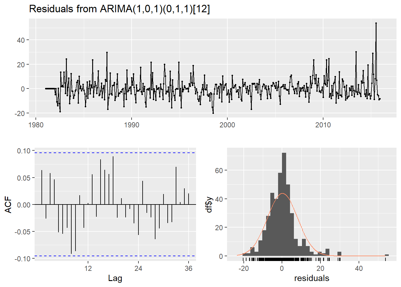
    Ljung-Box test

data:  Residuals from ARIMA(1,0,1)(0,1,1)[12]
Q* = 29.36, df = 21, p-value = 0.1056

Model df: 3.   Total lags used: 24
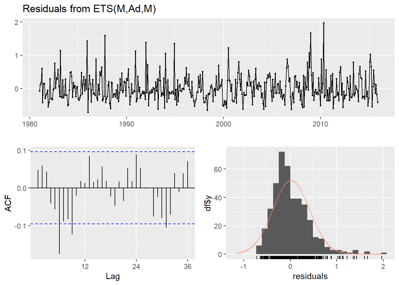
ETS model
    Ljung-Box test

data:  Residuals from ETS(M,Ad,M)
Q* = 43.792, df = 24, p-value = 0.008067

Model df: 0.   Total lags used: 24
Forecasting
Don't know how to automatically pick scale for object of type <ts>. Defaulting
to continuous.
Warning: Removed 11 rows containing missing values or values outside the scale range
(`geom_line()`).
Removed 11 rows containing missing values or values outside the scale range
(`geom_line()`).
Warning: Removed 420 rows containing missing values or values outside the scale range
(`geom_line()`).
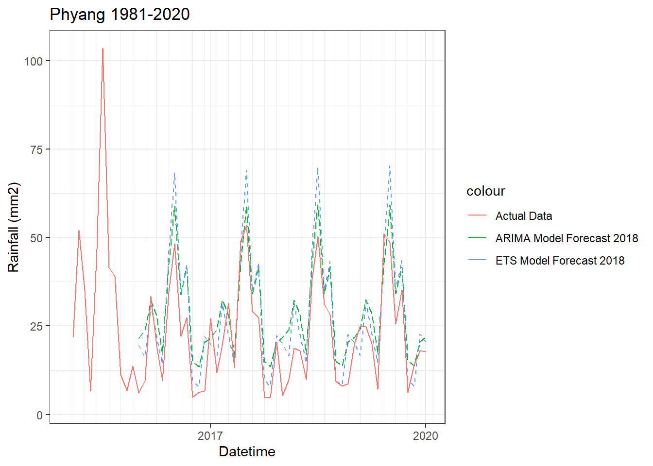
Accuracy of models
                    ME     RMSE       MAE        MPE     MAPE      MASE
Training set  0.170763  7.87356  5.388082  -9.139575 35.28552 0.8073011
Test set     -9.964325 10.87446 10.165830 -99.206968 99.81011 1.5231554
                     ACF1 Theil's U
Training set  0.063420750        NA
Test set     -0.004907483 0.9583204
                    ME     RMSE     MAE       MPE     MAPE      MASE       ACF1
Training set  0.285966  7.61933 5.34607 -13.12624 33.12538 0.8010065 0.02948987
Test set     -8.700370 10.85699 9.13186 -73.04490 74.33643 1.3682347 0.27990111
             Theil's U
Training set        NA
Test set     0.7923204
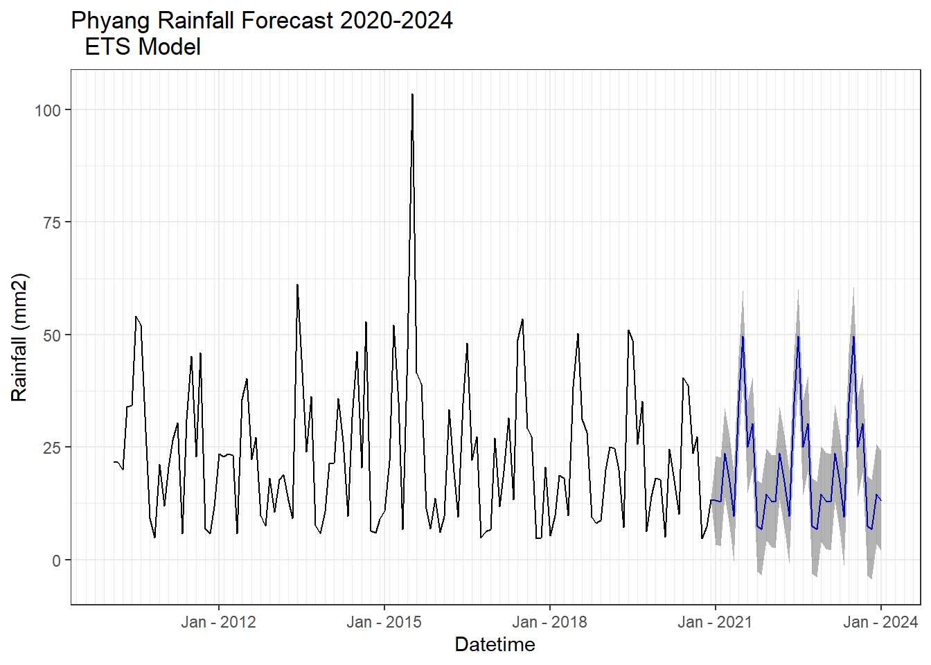
##Forecasting and plot
Warning: Removed 349 rows containing missing values or values outside the scale range
(`geom_line()`).
Warning: Removed 11 rows containing missing values or values outside the scale range
(`geom_line()`).
Warning: Removed 349 rows containing missing values or values outside the scale range
(`geom_line()`).
Removed 11 rows containing missing values or values outside the scale range
(`geom_line()`).